Matlab Tutorial for Beginners

Introduction to Matlab. How to begin Matlab.

MATLAB is a numerical computing environment and programming language. Created by The MathWorks, MATLAB allows easy matrix manipulation, plotting of functions and data, implementation of algorithms, creation of user interfaces, and interfacing with programs in other languages. Many classes in our ECEn Department requires professional skill using matlab, such as ECEn 360, ECEn 370, ECEn 380, ECEn 483...This tutorial is for those who never touch matlab before or need some review for matlab.
This flash will teach you how to start matlab in BYU ECEn Department.
1. Writer: Zixu Zhu
2. Email: sz_jamesrei@hotmail.com
The topics below are the most important topics selected from the result of students' survey.

Vectors, matrix and arrays

Setting up a vector or array
1. One dimension arrays and vectors are almost the same in Matlab. You can use either vector or array form to store variables.
2. Vector Format: x=a : b
3. Array Format (one dimensional): x= [a:b], a is the beginning value, b is the ending value, the default step is 1
4. For example
  1. a=[1:3], or a=1:3
  2. a is stored as: 1 2 3
5. If you want to change the step length, the format is: x=a:"length of step":b
6. For example:
  1. a=-1:0.5:1
  2. a is: -1.0000 -0.5000 0 0.5000 1.0000
7. Of course, you can also set each element by hand, using a space to separate each element in the row, and a semicolon to separate each row.
8. For example:
  1. a=[1 3 7 11;3 6 4 1]
  2. a will be:
  3. 1 3 7 11
  4. 3 6 4 1
Useful default arrays
1. Matlab has 2 useful default arrays: zeros, and ones. Each is an array filled with either zeros or ones. The format is : zeros/ones("number of dimension", length of array);
2. For example:
  1. a=zeros(1,3)
  2. a is stored as: 0 0 0
  3. a=ones(1,3)
  4. a is stored as: 1 1 1
3. With these two useful arrays, you can save time on setting values. For example, if you want to simulate a step function: x=[zeros(1,5) ones(1,5)], then x will be: 0 0 0 0 0 1 1 1 1 1
Operations between arrays
1. After setting the variables, you can do normal operations between arrays. To make an operation work on an array, just add a dot before the normal operator.
2. For example:
  1. a=1:4;
  2. b=a.^(1/2)
  3. the result will be: b = 0.5000 1.0000 1.5000 2.0000
3. or, you can also use b=sqrt(a), the result is same.
4. You don't need to set a for loop like in other programming languages to calculate the value of each element in b. Matlab will do it itself.
5. Another example:
  1. x=1:4;
  2. y=sin(x)+2.*x
  3. y will be: 2.8415 4.9093 6.1411 7.2432
P.S. Matrix operations are very similar to the array operations, detailed information can be found in the attached document.

Graphing

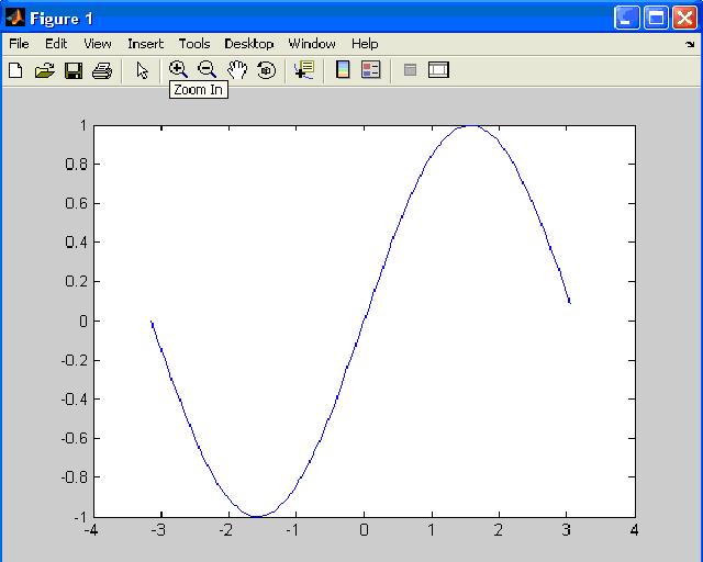
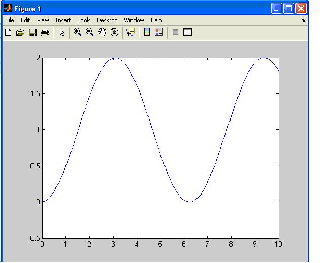
After setting and operating on arrays, the best way to see the behavior of x and y, or x,y, and z is to graph them. The most common functions for graphing are; plot, stem, polar, subplot, mesh, meshc, surf, surfc , and hold on.
plot and stem:
1. The format for these is the same. They both are: plot/stem(x,y).
2. The difference is: plot will plot a continuous graph; stem is for the discrete graph.
3. For example:
  1. x=-pi:0.1:pi;
  2. y=sin(x);
  3. plot(x,y)
  4. The result is:
  7. For stem(x,y) the result will be:
polar graph:
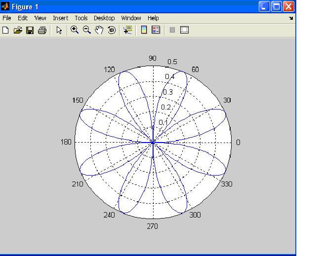
1. Occasionaly, polar graphs may be better to see the relation between 2 variables. In EcEn 360, to graph the signal of an antenna, using a polar function is useful.
2. Similar to plot and stem commands, the format for a polar graph is: polar(x,y).
3. p.s. In this case, x probably is always an angle with a range of 0 to 2pi.
4. For example:
  1. x=0:0.01:2*pi;
  2. y=sin(2*x).*cos(2*x);
  3. polar(x,y)
  4. The output will be:
3D graph:
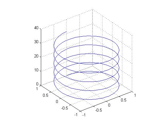
1. Some times we need to see the behavior of three variables. In EcEn 360, it's required to plot a 3D graph of the probability with two variables. There are many useful functions that can simulate 3D graphs depending on which one you need.
2. plot3:
  1. This function is mainly used for parametric functions, the syntax is: plot3(X1,Y1,Z1,...) where X1, Y1, Z1 are vectors or matrices. It will plot one or more lines in three-dimensional space through the points whose coordinates are the elements of X1, Y1, and Z1.
  2. For example:
    1. t = 0:pi/50:10*pi;
    2. plot3(sin(t),cos(t),t)
    3. grid on
    4. axis square
    5. the result will be:
3. mesh and surf:
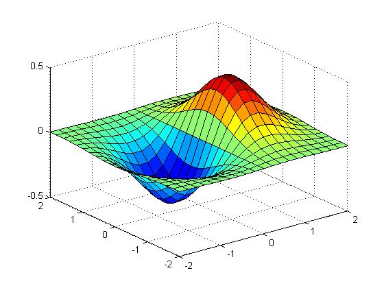
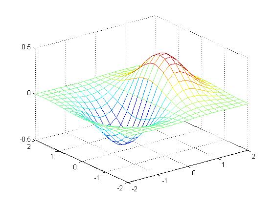
  1. The syntax for these two functions is very similar to plot3, both are: mesh/surf(x,y,z). The difference is that these two functions will output a surface graph instead of only the connections of the dots.
  2. For example:
    1. [X,Y] = meshgrid(-2:.2:2, -2:.2:2);
    2. Z = X .* exp(-X.^2 - Y.^2);
    3. surf(X,Y,Z)
    4. the output will be:
    7. if mech is replaced by surf, then the result will be:
    10. P.S. In this program, [X,Y] = meshgrid(x,y) transforms the domain specified by vectors x and y into arrays X and Y, which can be used to evaluate functions of two variables and three-dimensional mesh/surface plots. The rows of the output array X are copies of the vector x; columns of the output array Y are copies of the vector y.
4. meshc and view:
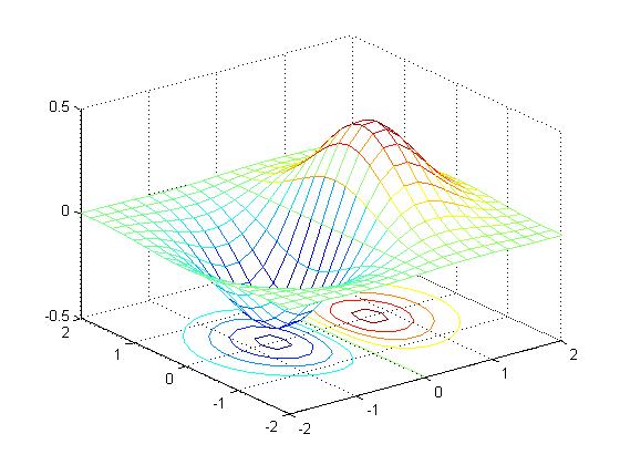
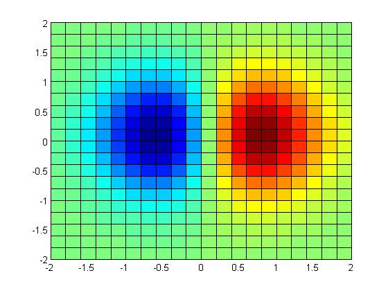
  1. These two functions will give you the idea of a 3D graph in a 2D one. "meshc" function will give you the contour plot of a 3D graph. "view(2)" will give you the view of a 3D graph when looking down from the top of it.
  2. For example:
    1. We can just add the "meshc(X,Y,Z)" at the end of last example to compare the results:
    2. [X,Y] = meshgrid(-2:.2:2, -2:.2:2);
    3. Z = X .* exp(-X.^2 - Y.^2);
    4. mesh(X,Y,Z)
    5. meshc(X,Y,Z)
    6. the result will be:
    9. Same for the view function:
    10. [X,Y] = meshgrid(-2:.2:2, -2:.2:2);
    11. Z = X .* exp(-X.^2 - Y.^2);
    12. surf(X,Y,Z)
    13. view(2)
    14. The result will be:

Derivative and Integration

Matlab can simulate both Integration and Derivative, not formulaically but by numerical approximation.
So, if you want a mathematical formula of a derivative, use a calculator or another program.
Derivative
1. Matlab is able to do differences and approximate derivatives, the basic function is diff.
2. The Syntax is: Y = diff(X) or Y = diff(X,n), n is the dimension of the derivative (such as a second derivative, third derivative, etc.) If n=1, it is the same as y=diff(x).
3. diff(x)
  1. y=diff(X) calculates differences between adjacent elements of X.
  2. If X is a vector, then diff(X) returns a vector, one element shorter than X, of differences between adjacent elements:y=[X(2)-X(1) X(3)-X(2) ... X(n)-X(n-1)]
  3. If X is a matrix, then diff(X) returns a matrix of row differences: [X(2:m,:)-X(1:m-1,:)]
  4. For example:
    1. x = [1 2 3 4 5];
    2. y = diff(x)
    3. result is: y = 1 1 1 1
  5. Furthermore, if the step in x is small enough, we can approximate its derivative:
  6. For example:
    1. step=0.001;
    2. x=0:step:2*pi;
    3. y=sin(x);
    4. z=diff(sin(x))/step;
    5. subplot(1,2,1);
    6. plot(y);
    7. subplot(1,2,2);
    8. plot(z);
    9. In this case, z is the derivative of y=sin(x), it should be cos(x)
    10. so from the plot we can see it is:
4. diff(X,n)
  1. Y = diff(X,n) applies diff recursively n times, resulting in the nth difference. For example, diff(X,2) is the same as diff(diff(X)). So for the first example above, if you type: z = diff(x,2) The result will be "z = 0 0 0"
Integral
1. Integrals work similar to derivatives. Matlab can also approximate implement integrals. There are many functions that can do this, such as: cumsum, trapz, quad, etc. The cumsum function is the most useful one.
2. The syntax is: B = cumsum(A). It returns the cumulative sum along different dimensions of an array. If A is a vector, cumsum(A) returns a vector containing the cumulative sum of the elements of A. If A is a matrix, cumsum(A) returns a matrix the same size as A containing the cumulative sums for each column of A.
3. For example:
  1. x=0:0.1:10;
  2. y=sin(x);
  3. z=cumsum(y)*0.1;
  4. plot(x,z)
  5. The result shows the integral of sin(x):

Signal processing

The number one important operation in simulating a system or signal is a convolution.
Before we look at a convolution, let's first simulate two very useful functions: the delta function and step function.
We can use long arrays storing zeros and ones to approximately simulate those two functions.
For example:
1. Impulse function:
  1. nx=-50:50;
  2. x=[zeros(1,50) 1 zeros(1,50)];
  3. plot(nx,x);
  4. The output will be:
2. Step function:
  1. nx=-50:50;
  2. x=[zeros(1,50) ones(1,51)];
  3. plot(nx,x);
  4. The plot of result will be:
Now, we can look at the convolution. The syntax is just like this: conv(f1,f2);
For example
1. Let's convolt these two functions:
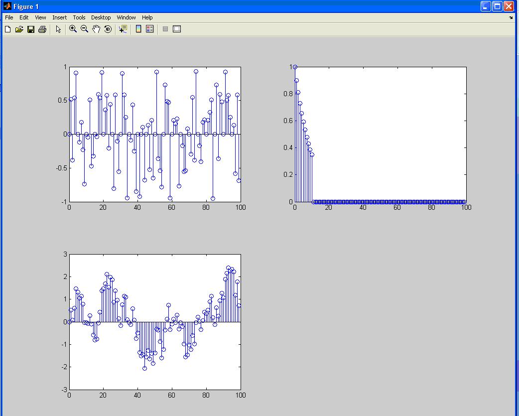
2. X=cos(n^2)*sin(2*pi*n/5)*u(t) and h=((0.9)^n)*(u(t)-u(t-10))
3. Then the code will be:
4. n=0:99;
5. unit=ones(1,100);
6. unit_10=[ones(1,11) zeros(1,89)];
7. h=((0.9).^n).*unit_10;
8. x=cos(n.^2).*sin(2*pi*n/5).*unit;
9. y=conv(x,h);
10. subplot(2,2,1);
11. stem(n,x);
12. subplot(2,2,2);
13. stem(n,h);
14. subplot(2,2,3);
15. stem(n,y(1:100));
16. The result is:
Filter and sampling processing will be taught in detail in ECEn380 class, you can also check it in the attached document.

Help and look for function

The Help function is the most useful function in Matlab. It lists all primary help topics in the Command Window. Each main help topic corresponds to a directory name on the MATLAB search path.
The Syntax of help function is:
help /
This command lists all operators and special characters, along with their descriptions.
help functionname
This command displays M-file help, which is a brief description and the syntax for functionname, in the Command Window. The output includes a link to doc functionname, which displays the reference page in the Help browser, often providing additional information. I think that doc link is the most useful link in Matlab. It should contains all you want to know.

A very convenient tool of MATLab 7.0 for graphing

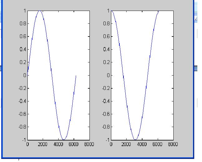
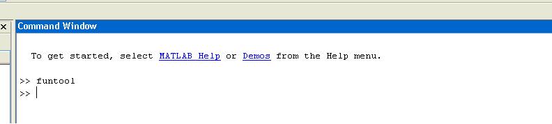
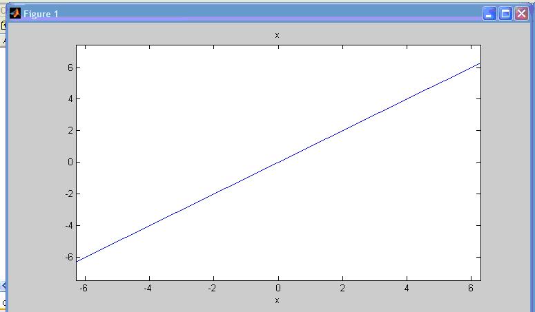
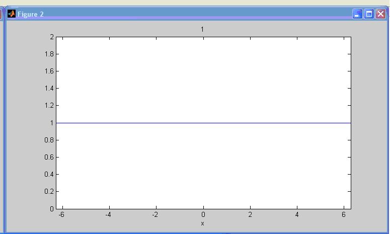
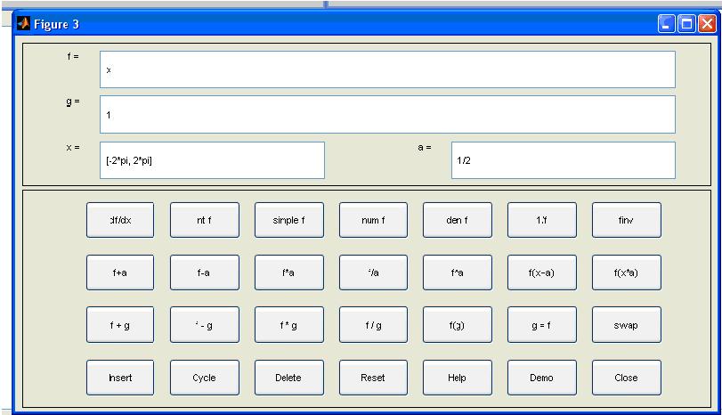
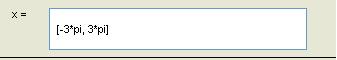
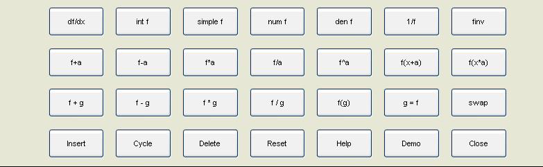
If you don't like coding and still want to see the behavior of a function or two functions, the easiest way to do that in MatLab 7.0 is using the "funtool" function.
First, type "funtool" in the Command Window like this:
Then, 3 windows(Figures) will show up (click image to enlarge):
These three images are the basis of the "funtool" function (click images to enlarge):
1.Figure 1:
1. It is the graph of function f which will be defined in Figure 3.
2.Figure2:
1. It is the graph of function g which will also be defined in Figure 3.
3.Figure3:
2. a.Function input windows:
  1. "f=": type in the expression of f function with variable x, the default expression is "x"
  2. Example for f=x^2:
  3. "g=": same as f function, type in the expression of g function , the default expression is "1"
  4. Example for g=sin(x):
3. b.Range of x window("x="):
  1. Input the range of x in "x=" window, the format is "[starting value, ending value]"
  2. For Example, if we want x from -3pi to 3pi:
4. c."a=" window:
  1. This is window is to set the value of "a" which is a factor of f. It may shift, shrink or enlarge the function f. The default value is ½.
5. d.operation panel
  1. As you see, you can do almost all the common opertions between these two functions or just one function itself. The result plot will show up in Figure 2 or Figure 3.